

The essential answer
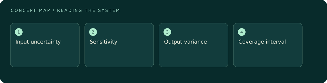
An uncertainty budget lists the important inputs to a measurement model, their estimated uncertainties, and how strongly each affects the result. Convert every contribution into the output unit before combining it. For independent inputs in a locally linear model, combine standard uncertainty contributions by summing their squares and taking the square root. Correlated inputs require covariance terms. The budget is a structured statement of what is known about the result, not a list of every imaginable problem or a substitute for correcting known effects.
How to reason about it
Write y = f(x1, x2, …) and evaluate sensitivity coefficients at the operating point. A voltage uncertainty, for example, becomes a force contribution through the inverse sensitivity. Repeatability can supply one contribution, while calibration records, finite resolution, environmental corrections, and geometric tolerances supply others. Their origin does not determine whether they are systematic or random in a particular sequence. State assumed distributions and convert quoted limits or expanded uncertainties into standard uncertainties consistently. Check whether linear propagation is adequate: strong nonlinearity, bounds, or asymmetric inputs may call for numerical propagation and a non-symmetric interval. Rank the resulting variance contributions to guide improvement. A carefully estimated small contribution is not where effort belongs if one poorly known thermal coefficient dominates the outcome. Keep model inadequacy visible instead of hiding it inside an arbitrary safety factor.
ILLUSTRATIVE · NOT A REPORTED RESULT
An example to work through
Assume independent illustrative force contributions of 0.20 nN from calibration, 0.10 nN from repeatability, and 0.30 nN from baseline interpolation. Their combined standard uncertainty is sqrt(0.20²+0.10²+0.30²) = 0.374 nN. With a justified coverage factor k = 2, expanded uncertainty is 0.748 nN, conventionally rounded to 0.75 nN. Baseline interpolation contributes 0.09/0.14 = 64.3% of the total variance. Halving repeatability alone barely helps; halving the baseline contribution gives sqrt(0.04+0.01+0.0225) = 0.269 nN, identifying the more useful improvement. All quoted uncertainty components here are standard uncertainties.
Where interpretation fails
Adding a “systematic error” line without a model can conceal double counting. A temperature fluctuation may already appear in observed repeatability and also be included through a temperature coefficient. Determine what each contribution represents and whether the same variation has already entered another term before combining them.
The next decision
Use the budget to decide whether a planned change can meet a target uncertainty. Recalculate the total after changing the dominant contribution, and include any new terms introduced by the redesign. Report coverage factors and assumptions so the numerical interval can be interpreted consistently across experiments and comparisons.
Sources & context
These sources support the concepts noted below. Our synthetic examples and research framing are educational interpretation; they are not findings from these organizations or validation of our ventures.
- JCGM 100: Guide to uncertainty ↗
Further reading on uncertainty propagation; PDF text inspected, not a full document review.
Source check: Relevant excerpt or resource metadata checked; see support note. Original illustrative calculation, not source data.
Educational research context, not a validated device specification or clinical protocol. Read our editorial and correction policy.