

The essential answer
Uncertainty propagation translates uncertainty about inputs into uncertainty about a model output. It requires a defined model, input estimates, and information about their variability and dependence. For small perturbations in a smooth model, local sensitivities provide a useful approximation. Nonlinear or bounded problems may require sampling or another method that preserves the input structure. The resulting interval is conditional on the supplied model and uncertainty description. It cannot automatically include unknown mechanisms, unrecognized biases, or operating conditions that were absent from the analysis.
How to reason about it
Write the output as a function of explicitly named inputs. Distinguish repeated-measurement variability from uncertainty in calibration factors and other shared quantities. A shared calibration error affects many observations together and will not vanish merely by averaging more readings. Covariance matters because two inputs can reinforce or cancel each other's influence. Before applying a local formula, inspect whether the expected input range crosses a nonlinear region, a bound, or a discontinuity. If sampling is used, generate inputs from a justified joint distribution rather than independent distributions chosen for convenience. Check numerical convergence of the propagated summaries and retain the sampling seed and configuration. Report the output estimate together with the meaning of the uncertainty measure, such as a standard uncertainty or a stated coverage interval. Separately discuss model discrepancy when the mathematical relationship is only an approximation to the real measurement process.
ILLUSTRATIVE · NOT A REPORTED RESULT
An example to work through
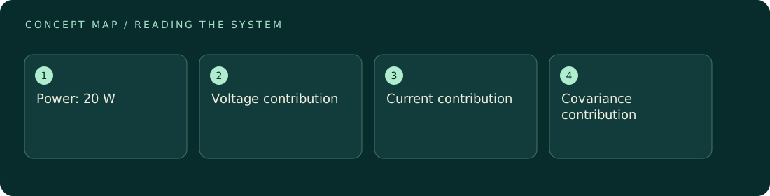
Assume electrical power is P = VI, with estimates V = 10 V and I = 2 A. Let standard uncertainties be 0.1 V and 0.02 A, and initially assume they are uncorrelated. The first-order variance is I squared times 0.1 squared plus V squared times 0.02 squared = 0.04 + 0.04 = 0.08 W squared. Standard uncertainty is therefore about 0.283 W around 20 W. If the correlation coefficient is 0.5, the covariance contribution adds 0.04 W squared, raising standard uncertainty to about 0.346 W. These are constructed inputs illustrating the effect of dependence.
Where interpretation fails
Adding all uncertainty percentages linearly and calling the result a standard uncertainty mixes a worst-case style bound with a probabilistic quantity. The opposite error is combining everything in quadrature without checking independence. Both can misrepresent confidence when common calibration or environmental effects correlate the inputs.
The next decision
Use a first-order calculation when the model is smooth over the plausible input range and validate that approximation when the decision is sensitive. Preserve covariance or joint samples whenever dependence matters. If the resulting uncertainty overlaps a decision threshold, improve the dominant information source or adopt an explicit decision rule for that overlap.
Sources & context
These sources support the concepts noted below. Our synthetic examples and research framing are educational interpretation; they are not findings from these organizations or validation of our ventures.
- NIST: Combining uncertainty components ↗
First-order uncertainty propagation uses sensitivity coefficients and covariance.
Source check: Official HTML opened; propagation conditions inspected.
Educational research context, not a validated device specification or clinical protocol. Read our editorial and correction policy.