

The essential answer
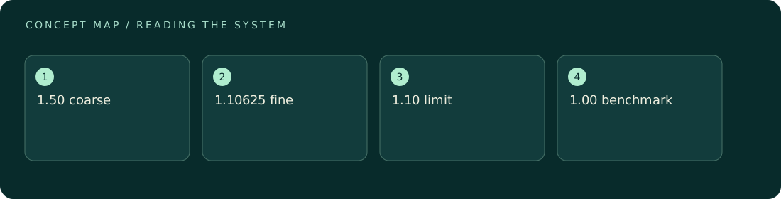
An illustrative grid sequence approaches 1.10 while the intended benchmark is 1.00. Refinement steadily removes the h² discretization term, but a fixed 0.10 model offset remains. The computed answer can look increasingly stable while retaining a ten-percent discrepancy. Convergence therefore supports a statement about numerical consistency within a model; it does not by itself validate boundary conditions, constitutive assumptions, implementation choices, or agreement with the physical quantity of interest.
How to reason about it
Represent the computed quantity as Q(h)=Qtrue+b+ah², with grid scale h, fixed bias b, and a leading second-order discretization term. Reducing h shrinks only the last term. Richardson-style reasoning can estimate the limiting value for this family, but that limit includes b. A plateau may alternatively result from iterative tolerance, roundoff, or insufficient precision, so the cause needs investigation. The NASA tutorial addresses spatial convergence as a tool for estimating discretization error. The synthetic offset in this example deliberately lies outside that target. A robust interpretation asks both whether numerical error is controlled and whether the modeled quantity, equations, and conditions represent the intended benchmark or experiment.
ILLUSTRATIVE · NOT A REPORTED RESULT
An example to work through
Choose illustrative Qtrue=1.00, b=0.10, and a=0.40. At h=1, Q=1.50. At h=0.5, Q=1.20. At h=0.25, Q=1.125. At h=0.125, Q=1.10625. Successive changes are 0.30, 0.075, and 0.01875, each smaller by a factor of four, as expected for h² scaling under halving. Using the last two grids, the second-order extrapolation is Qext=Qfine+(Qfine−Qcoarse)/(4−1)=1.10625−0.01875/3=1.10. The extrapolation correctly removes the remaining 0.00625 discretization contribution on the finest grid, yet still differs from Qtrue by 0.10. Relative to the benchmark, that is 10 percent. If acceptance required agreement within 1 percent, numerical convergence would not satisfy the requirement. The example gives an exact analytic error model so the distinction is visible; real error orders and asymptotic ranges must be assessed rather than assumed from a short sequence.
Where interpretation fails
A small difference between two grids can be caused by cancellation or a shared error, not just high accuracy. Reporting many stable digits reinforces the wrong impression. Also avoid using an assumed convergence order when the grids are not in the asymptotic regime or the solution contains unresolved features.
The next decision
Use the refinement sequence to bound discretization effects, then compare the extrapolated result with independent benchmarks and conservation checks. Here the appropriate conclusion is convergence toward 1.10 with unresolved model disagreement. Tightening the grid alone cannot remove the constructed constant offset, so further refinement is not the key next investigation.
Sources & context
These sources support the concepts noted below. Our synthetic examples and research framing are educational interpretation; they are not findings from these organizations or validation of our ventures.
- NASA: Examining Spatial Grid Convergence ↗
Grid refinement assesses discretization error, which differs from other errors.
Source check: Official convergence tutorial introduction read
Educational research context, not a validated device specification or clinical protocol. Read our editorial and correction policy.