

The essential answer
Timestep convergence tests whether a transient prediction changes acceptably as the time increment is reduced. Numerical stability only means that the method avoids a particular form of growing numerical failure; it does not guarantee accurate phase, peak amplitude, or event timing. Compare the same physical observable over the same time interval with spatial error and iterative error controlled. A single final value can hide an inaccurate trajectory, so include the transient features that matter to the engineering or scientific conclusion.
How to reason about it
First identify the fastest dynamics that the requested output must resolve. That may be a short pulse, a contact event, a transport time, or an oscillation rather than the overall duration of the simulation. Refine the time increment while keeping input interpolation, event rules, and output sampling consistent. Distinguish the solver timestep from the frequency at which results are saved: fine integration with coarse saved output can still miss the peak used in a report. Adaptive solvers need tolerance studies and recorded accepted steps rather than a claim based only on a nominal step setting. Compare values at aligned physical times or use a defined event metric when trajectories shift. If a spatially refined model introduces faster modes, repeat the temporal assessment because a timestep adequate for the original mesh may no longer resolve the new dynamics.
ILLUSTRATIVE · NOT A REPORTED RESULT
An example to work through
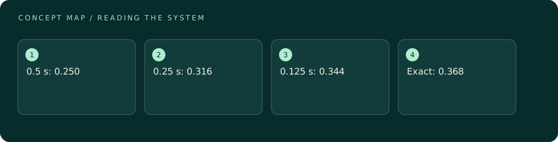
Assume an ideal decay y prime = -y with y(0) = 1 and time measured in seconds. Forward Euler with step 0.5 s gives y(1) = 0.5 squared = 0.25. With 0.25 s it gives 0.75 to the fourth power = 0.31640625. With 0.125 s it gives 0.875 to the eighth power, approximately 0.343609. The exact value is exp(-1), approximately 0.367879. All three numerical sequences decay without exploding, yet their one-second predictions differ substantially. The example demonstrates stability without sufficient accuracy and shows the expected improvement as this first-order method is refined.
Where interpretation fails
Reducing the saved-output interval without changing integration accuracy can create a smoother-looking curve without a more accurate solution. Another common error is judging an oscillatory simulation only by its final amplitude, even though a phase error has shifted every load peak and could change the predicted response.
The next decision
Accept a time discretization only against tolerances for the actual transient outputs: peak, integral, settling time, or another defined measure. If refinement changes event order or peak location materially, investigate the time integration and event handling before using the result. Preserve both integration settings and output sampling settings with the run.
Sources & context
These sources support the concepts noted below. Our synthetic examples and research framing are educational interpretation; they are not findings from these organizations or validation of our ventures.
- NASA: Verification Assessment ↗
Consistency, temporal convergence, and independent numerical methods are verification checks.
Source check: Official tutorial opened; verification process inspected.
Educational research context, not a validated device specification or clinical protocol. Read our editorial and correction policy.