

The essential answer
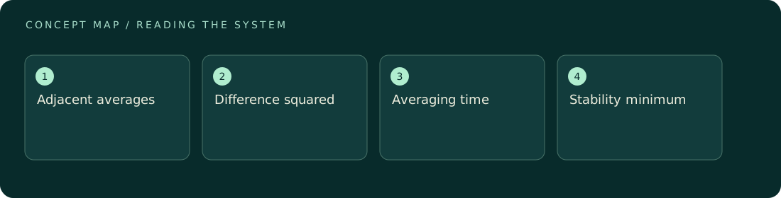
Allan deviation measures the typical difference between adjacent averages at a chosen averaging time. It is useful when ordinary sample variance hides time-dependent stability. For a sequence of averages x̄i of duration τ, a basic estimator is the square root of half the mean squared successive difference. Plotting it against τ shows where additional averaging helps and where slower variations begin to dominate. It is a stability diagnostic, not automatically the standard uncertainty of the final mean or a complete uncertainty budget.
How to reason about it
Specify whether the data represent frequency, phase, displacement, or another quantity, and choose the estimator accordingly. Frequency stability conventions often use fractional frequency, while a force record can be analyzed directly in force units with a clearly stated construction. White, uncorrelated sample noise typically averages down, but drift and correlated processes change the slope. Finite records provide few independent comparisons at long averaging times, so apparent minima there may be poorly established. Gaps, filtering, overlapping estimates, and dead time also affect interpretation. Use the curve to design switching and averaging, then validate that choice with independent runs. If detrending is applied, show the reason and preserve the original curve: removing drift changes the question being answered. An optimum from one quiet session may not transfer to a later environmental state or a different sampling configuration.
ILLUSTRATIVE · NOT A REPORTED RESULT
An example to work through
Consider illustrative adjacent ten-second force averages of 1, 3, 2, and 4 nN. Their differences are 2, −1, and 2 nN; the mean square difference is (4+1+4)/3 = 3 nN². The basic Allan deviation is sqrt(3/2) = 1.225 nN. This tiny sample is only an arithmetic demonstration, not a robust stability estimate. If a much longer real record showed decreasing deviation to 30 seconds and rising deviation beyond that, a 30-second averaging window would be a candidate to test, rather than an automatically optimal protocol.
Where interpretation fails
Do not read the lowest plotted point as a guaranteed uncertainty floor. Long averaging times contain fewer effective samples, and deterministic disturbances can create misleading structure. Also avoid converting stability directly into absolute accuracy: a constant calibration bias contributes no adjacent-average difference and can remain invisible.
The next decision
Use Allan deviation when timing choices materially affect noise rejection. Require enough data to support the chosen timescale, retain estimator details, and confirm the selected window in a separate acquisition. Combine the resulting statistical information with calibration and systematic contributions before assigning uncertainty to the final measurement result.
Sources & context
These sources support the concepts noted below. Our synthetic examples and research framing are educational interpretation; they are not findings from these organizations or validation of our ventures.
- NIST Handbook of Frequency Stability Analysis ↗
Further reading on stability statistics; publication summary checked.
Source check: Relevant excerpt or resource metadata checked; see support note. Original illustrative calculation, not source data.
Educational research context, not a validated device specification or clinical protocol. Read our editorial and correction policy.