

The essential answer
Boundary conditions specify how the modeled region interacts with its surroundings. Together with governing equations, material relations, and initial conditions, they define the problem being solved. A sophisticated solver cannot recover information that was imposed incorrectly at an inlet, wall, support, or external surface. Separate physically measured boundary information from convenient numerical approximations. Then test the approximations that could influence the target observable. Boundary sensitivity should be assessed independently of mesh refinement because an increasingly accurate solution of the wrong boundary problem remains unsuitable.
How to reason about it
Begin by identifying what crosses each boundary: mass, momentum, energy, charge, displacement, or another conserved quantity. Decide whether the available evidence supports prescribing a value, a flux, or a relation between the two. Avoid imposing independent values that overconstrain the mathematical problem. Artificial boundaries require an additional question: is the truncated domain far enough from the process of interest, and does its numerical treatment allow the expected behavior? For a support in a structural calculation, compare a rigid fixture assumption with a plausible compliance. For thermal work, compare fixed surface temperature with finite heat transfer when the surroundings cannot maintain a perfect reservoir. The purpose is not to sweep arbitrary settings until an answer looks right. It is to connect alternative boundary descriptions to uncertainty about the real apparatus and report their influence on the chosen result.
ILLUSTRATIVE · NOT A REPORTED RESULT
An example to work through
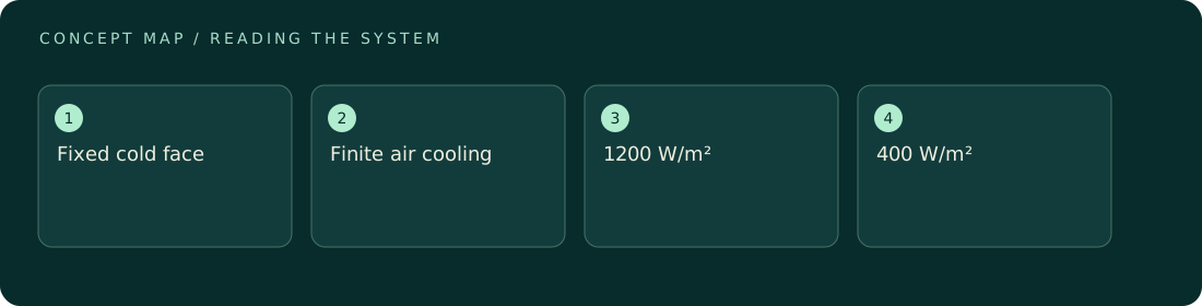
Assume steady one-dimensional conduction through a 0.1 m slab with conductivity 2 W/(m K). Holding its faces at 80 and 20 degrees Celsius predicts heat flux 2 times 60/0.1 = 1200 W per square metre. Suppose instead the cold side exchanges heat with 20-degree air through a coefficient of 10 W/(square metre K). The total resistance per area is 0.1/2 + 1/10 = 0.15 square metre K/W, so flux is 60/0.15 = 400 W per square metre. The cold surface is then 60 degrees Celsius. This idealized example changes only the boundary model and produces a threefold flux difference.
Where interpretation fails
Agreement between two meshes is sometimes mistaken for agreement with the apparatus. Both meshes may enforce the same unrealistic temperature or displacement. Another trap is moving an outlet while simultaneously changing turbulence settings or mesh quality; the resulting difference cannot then be attributed cleanly to boundary placement.
The next decision
Prioritize a boundary study when inputs at the domain edge are uncertain or the result changes strongly near that edge. Keep the equation set and numerical controls fixed during the comparison. If boundary uncertainty exceeds the design margin, obtain better boundary measurements or explicitly widen the prediction interval before deciding.
Sources & context
These sources support the concepts noted below. Our synthetic examples and research framing are educational interpretation; they are not findings from these organizations or validation of our ventures.
- Slater: Verification Assessment of Flow Boundary Conditions ↗
Boundary implementations require verification against suitable reference problems.
Source check: NASA bibliographic abstract opened; full paper not reviewed.
Educational research context, not a validated device specification or clinical protocol. Read our editorial and correction policy.