

The essential answer
Mesh convergence asks whether a numerical prediction approaches a stable limit as spatial resolution improves. Choose the quantity that matters to the decision, refine systematically, and measure how that quantity changes. At least three suitably related resolutions are often useful for diagnosing the trend rather than merely observing one difference. A finer mesh is not automatically more trustworthy if geometry, boundary treatment, solver tolerances, or model settings also change. Convergence supports control of spatial numerical error within the chosen mathematical model; it does not establish that the model represents the experiment.
How to reason about it
Define a mesh family that improves the features responsible for the output, including near-wall gradients, interfaces, or local stress concentrations. State a representative spacing and its relationship between levels. Solve each case tightly enough that iterative error does not dominate the spatial comparison. Plot the output against spacing or an appropriate power of spacing and inspect whether successive differences shrink in a consistent way. Nonmonotonic behavior, moving discontinuities, and singular quantities require special care; a maximum stress at an ideal sharp corner may not possess the finite limit being sought. In such cases choose a physically meaningful averaged quantity or revisit the geometry. A convergence report should preserve mesh generation settings and output extraction details, because two people can obtain different apparent trends simply by sampling at different locations. Budget computational effort around the accuracy needed for the actual decision.
ILLUSTRATIVE · NOT A REPORTED RESULT
An example to work through
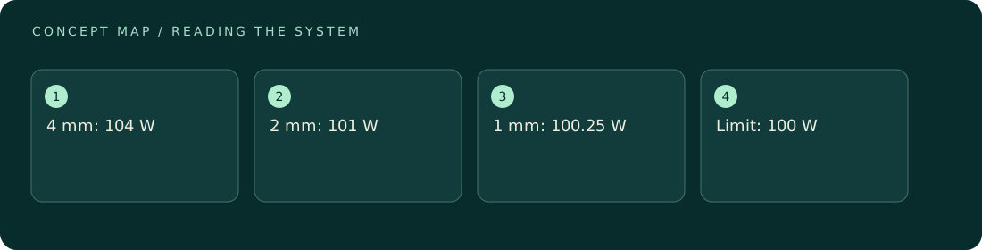
Consider invented heat-flow results on meshes with spacing 4, 2, and 1 mm: 104, 101, and 100.25 W. Successive changes are 3 and 0.75 W, a ratio of four for a spacing ratio of two. Under an asymptotic power-error assumption this is consistent with second-order convergence. Extrapolation gives 100.25 + (100.25 - 101)/(4 - 1) = 100 W. The estimated fine-mesh correction is 0.25 W, or about 0.25 percent of the extrapolated value. This neat sequence illustrates the calculation only; a real study must check whether its refinement behavior supports the assumed error model.
Where interpretation fails
Reporting millions of cells is not an accuracy statement. Local resolution can remain inadequate in the region controlling the output. Nor does a small change between two meshes prove convergence: numerical errors can cancel or the pair can sit outside the range where the expected refinement law applies.
The next decision
Stop refining when the estimated spatial contribution is comfortably below a predetermined decision tolerance and the observed trend is credible. Continue if the output is nonmonotonic or the remaining correction could reverse the decision. Report the estimate and its assumptions rather than describing the final mesh as simply independent of resolution.
Sources & context
These sources support the concepts noted below. Our synthetic examples and research framing are educational interpretation; they are not findings from these organizations or validation of our ventures.
- NASA: Examining Spatial Convergence ↗
Refinement studies assess observed numerical convergence.
Source check: Official tutorial opened; order and asymptotic convergence sections inspected.
Educational research context, not a validated device specification or clinical protocol. Read our editorial and correction policy.